Monday, April 21, 2014

A Reply to "Does Inflation Make You Poorer?"

Noah Smith channels Robert Shiller circa 1997 in his recent post, "Does Inflation Make you Poorer?" While Noah asks this question rhetorically, Shiller actually asked a series of related questions in a questionnaire of 677 people. His sample included both economists and non-economists from the U.S., Brazil, and Germany. He found:
"Among non-economists in all countries, the largest concern with inflation appears to be that it lowers people’s standard of living. Non-economists appear often to believe in a sort of sticky-wage model, by which wages do not respond to inflationary shocks, shocks which are themselves perceived as caused by certain people or institutions acting badly. This standard of living effect is not the only perceived cost of inflation among non-economists: other perceived costs are tied up with issues of exploitation, political instability, loss of morale, and damage to national prestige."
The first concern is the subject of Noah's mockery. True, some people think in partial equilibrium, neglecting the effects that inflation might have on their nominal income. But it is not an unreasonable concern in some contexts. Nominal wage stagnancy is a reality for many workers. In a 2008 Pew Survey, 57% of respondents believed that their income was rising slower than the cost of living.

In the figure below, the CPI, average hourly earnings for all private sector workers, and average hourly earnings for retail trade employees are all plotted. All are normalized to 100 in 2006. While average hourly earnings for all workers have grown faster than the CPI, the opposite is true for workers in retail. Since 2006, the price level is about 21% higher, but hourly wages in retail are less than 11% higher. They feel poorer and they are poorer.

Did inflation "make them poorer?" Not directly. But the political economy of inflation certainly contributed. Prices and wages do not simply rise or fall on their own. People choose to raise or lower them--this is why prices and wages are in the domain of economics, after all. Who chooses, and how do they choose? That's where things get more complicated. Decision-makers at firms set prices subject to an almost innumerable set of constraints and considerations imposed by the institutional and policy environment they face. Wages are not simply set by some abstract market-clearing condition; they involve bargaining between firms and individual employees or labor unions. Regulations, policy, and social norms also affect the bargaining powers of the relevant groups, with palpable effects on the wage structure.

Source: http://research.stlouisfed.org/fred2/graph/?g=y1d

In Japan, for example, deflation has plagued the economy for years. When Shinzo Abe ushered in a return to positive inflation, most Japanese consumers described rising prices as "rather unfavorable." These consumers were not being unreasonable. They were getting poorer! When prices started rising, wages did not. Since the 1950s, Japanese salaries have been determined by coordinated negotiations between unions and large employers. Only very recently, with the backing of Abe, have the unions had sufficient bargaining power to raise salaries in these negotiations. Japan also has a growing informal sector, where already-low nominal wages are unlikely to rise with the price level. Maybe eventually the overall Japanese economy will grow so much that even the low-wage informal workers will be better off. But no one knows how long that could take. Noah says it himself: "Whenever you buy something, the money you spend is someone else's income." But we don't know whose income it will be.

This is not to say that Japanese deflation was a good thing or made people richer. Quite the opposite. But it is to say that people should complain when their cost of living is rising faster than their earnings. Inflation has distributional effects, which will tend to benefit the politically powerful. The people getting the short end of the deal are perfectly rational to be upset about it, especially if their dissatisfaction can be harnessed into political action.

Not only inflation itself, but also inflation risk, has costs and distributional effects. The unpredictability of inflation is part of its cost. Hedging against inflation is theoretically possible but difficult. Inflation risk is costly for its bearers. Our political and economic institutions determine who the bearers will be. When social security and pensions are indexed to the price level, inflation risk to pensioners is reduced, while inflation risk to pension funds increases. When private debt contracts are primarily nominal, an unexpected increase in inflation will be costly for creditors. Indexing sovereign debt to the price level also redistributes inflation risk between countries and their creditors.

The other perceived costs of inflation that Shiller lists--exploitation, political instability, loss of morale, and damage to national prestige--all have historical precedents and are also related to the political economy of inflation. A government that "inflates away its debts" risks imposing any or all of these costs.  These costs of inflation are less relevant in the low inflation environments of the United States and much of Europe today. An increase in inflation from, say, 1% to 3% is unlikely to foster political instability or erode national prestige.

In the U.S. today, I think a little more inflation would be a good thing. But I think we also should take seriously the concerns of people whose real income is falling for one reason or another. This boils down to another call for economists to keep worrying about inequality-- even when thinking about issues like inflation.

Thursday, April 10, 2014

Guest Post by John Mondragon: Keeping Up with the Joneses and Household Debt

This guest post was contributed by John Mondragon, an economics PhD candidate at Berkeley. He is the coauthor of a working paper that is closely related to my recent post on consumption contagion and income inequality. I'm very excited that he has agreed to contribute this post about the working paper. John is on Twitter @Mondragon_John

Since the 1980s U.S. households have dramatically increased the amount of debt they hold. One frequent explanation for this trend is that the large increase in income inequality over this same period caused households to borrow more (see Figure 1). The intuition is that low-income households attempted to “keep up” with the increasing consumption of their high-income neighbors. This could affect debt levels if the low-income household decides to fund its consumption by leveraging with debt (as opposed to increasing labor supply or drawing down assets). This type of behavior is often referred to as “keeping up with the Joneses”, consumption cascades, consumption spillovers, or external habit.

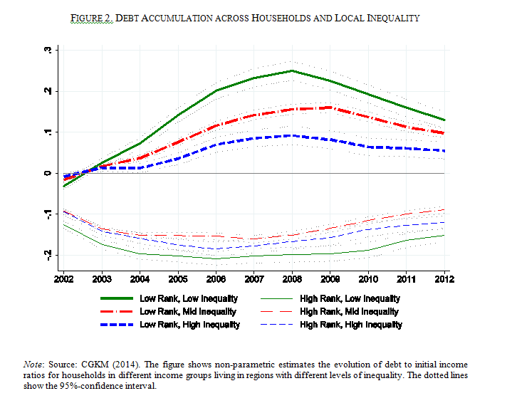
In a working paper I have with Olivier Coibion, Yuriy Gorodnichenko, and Marianna Kudlyak we look at whether, in the years running up to the financial crisis as well as during the Great Recession, low-, middle-, and high-income households accumulated different amounts of debt (relative to their incomes)  depending on the level of income inequality in their region. Our main finding is that low-income households in high-inequality areas increased their leverage by less than similar households in low-inequality areas. Our non-parametric results in Figure 2 suggest that a household in the bottom third of the income distribution within their area and inequality distribution across areas increased their leverage by around 15 percentage points more than a similar household in the top third of the inequality distribution in the years immediately prior to the financial crisis. This is the exact opposite effect one would expect if “keeping up with the Joneses” was the primary cause of borrowing by low-income households.

Because our data (see Additional Details below) allow us to break debt into pieces, we can examine which types of debt are driving these differences. While we find similar patterns for mortgage debt, auto debt, and credit card limits as those documented for total debt accumulation, we find no systematic differences across households and inequality regions in terms of their credit card balances. Since credit card limits primarily reflect credit supply conditions whereas credit card balances reflect households’ demand for credit, we interpret the difference in results across credit card limits and balances as pointing toward credit supply factors as the root cause of the link between inequality and borrowing.

The intuition is simple. First, lenders confront asymmetric information as they try to infer which borrowers are less likely to default. Second, high-income borrowers are less likely to default so lenders use income as a way to infer borrower type. In a perfectly equal income distribution all borrowers are equally likely to be a high or low default risk. But as inequality increases and the income difference between low- and high-income borrowers becomes larger, high-risk and low-risk borrowers are easier to tell apart when they reveal their incomes to banks. Lenders will then be able to offer cheaper and more readily accessible credit to high-income/low-risk borrowers as well as more likely to deny loans to low-income/high-risk borrowers. To test these predictions we use data from the Home Mortgage Disclosure Act (HMDA) which requires mortgage lenders to report details on applications including whether a loan was denied, the size of the loan, income of the applicant, and other characteristics. We find that low-income applicants are more likely to be denied mortgages and to be charged a high interest rate in high-inequality areas relative to similar applicants in low-inequality areas. Thus, this evidence also supports a credit supply interpretation of the link between local income inequality and differential borrowing patterns across income groups that is at odds with the “keeping up with the Joneses” interpretation.

Part of the reason I was invited to write here was to discuss the differences between our results and those in a recent paper by Bertrand and Morse, because their empirical findings do provide evidence of “keeping up with the Joneses” forces. There are at least two important differences. First, their outcome is consumption while ours is debt. It is possible that low-income households funded their consumption with changes in labor supply, savings, or even some debt. But our results tell us that any use of debt in this way cannot be the primary story of inequality and debt accumulation during this period. This is important to note because debt accumulation was central to the creation of many of the financial assets behind the financial crisis. Second, Bertrand and Morse use changes in consumption among the wealthy as their explanatory variable while we use inequality. It is possible that in some areas the consumption differences between households are not as large as in other areas even though both have the same measured inequality. This can occur if there is variation in precautionary savings, the “visibility” of consumption bundles, or the proximity of high- and low-income households. As the relationship between high-income household consumption and measured inequality becomes more complex our results become less directly comparable.

Thanks very much to Carola for having us!


Additional Details

The data we use for our primary results are from the New York Federal Reserve Bank Consumer Credit Panel/Equifax (referred to as the CCP), which provides comprehensive debt measures for millions of U.S. households since 1999. Because these data do not include income we impute incomes using the relationship between common observables in the Survey of Consumer Finances. Using these imputed incomes we construct measures of local inequality, household positions in the income distribution, and household debt-to-income ratios. We are able to check our measures of inequality and rank against various external measures and find they are very highly correlated.

Our results are robust to the level at which we measure inequality (zip, county, state), the measure of inequality we use (ratio of log incomes at the 90th and 10th percentile from the CCP, Gini coefficients from the IRS and Census data), an extensive set of household and area controls, and numerous splits of our sample. In particular our results hold within subsamples defined according to house price appreciation, average credit scores, income levels, initial debt ratios, and geographic regions.